Neutrino Cross Sections
Plot the cross sections for the key in-ice interactions for ~10 MeV neutrinos in IceCube.
[1]:
from asteria import interactions
from snewpy.neutrino import Flavor

import astropy.units as u
from astropy.table import Table

import numpy as np
import matplotlib as mpl
import matplotlib.pyplot as plt

from importlib.resources import files

from itertools import cycle
Setup styles for Plotting
[2]:
axes_style =   {            'grid' : 'True',
                       'labelsize' : '24',
                        'labelpad' : '8.0' }

xtick_style =  {       'direction' : 'out',
                       'labelsize' : '20.',
                      'major.size' : '5.',
                     'major.width' : '1.',
                   'minor.visible' : 'True',
                      'minor.size' : '2.5',
                     'minor.width' : '1.' }

ytick_style =  {       'direction' : 'out',
                       'labelsize' : '20.',
                      'major.size' : '5',
                     'major.width' : '1.',
                   'minor.visible' : 'True',
                      'minor.size' : '2.5',
                     'minor.width' : '1.' }

grid_style =   {           'alpha' : '0.75' }
legend_style = {        'fontsize' : '16' }
font_syle =    {            'size' : '20'}
text_style =   {          'usetex' : 'True' }
figure_style = {  'subplot.hspace' : '0.05' }

mpl.rc(    'font', **font_syle )
mpl.rc(    'text', **text_style )
mpl.rc(    'axes', **axes_style )
mpl.rc(   'xtick', **xtick_style )
mpl.rc(   'ytick', **ytick_style )
mpl.rc(    'grid', **grid_style )
mpl.rc(  'legend', **legend_style )
mpl.rc(  'figure', **figure_style )

mpl.rcParams['text.usetex'] = True
# mpl.rcParams['text.latex.preamble'] = [r'\usepackage[cm]{sfmath}']
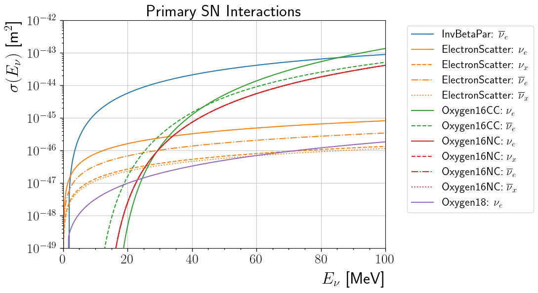
Neutrino Interactions
There are several important neutrino interactions to consider:
Inverse beta decay: \(\bar{\nu}_e+p \rightarrow e^{+} + n\).
Elastic neutrino scattering: \(\nu_e + e^{-} \rightarrow \nu_e + e^{-}\) (plus antineutrino, plus \(\mu\) and \(\tau\)).
Oxygen-16 charged-current interaction: \(\nu_e + ^{16}\mathrm{O}\rightarrow e^{-} + \mathrm{X}\) (plus antineutrino).
Oxygen-16 neutral-current interaction: \(\nu_\mathrm{all} + ^{16}\mathrm{O} \rightarrow \nu_\mathrm{all} + \mathrm{X}\).
Oxygen-18 interactions: \(\nu_e + ^{17/18}\mathrm{O} / ^{2}_{1}\mathrm{H} \rightarrow e^{-} + \mathrm{X}\).
For details, see R. Abbasi et al., A&A 535:A109, 2011.
NOTE (3/13/19): Inverse Beta Decay has two implentations in ASTERIA, InvBetaTab() and InvBetaPar(). Below the latter is shown, but comparison plots are generated for both.
[3]:
Interactions = [ interactions.InvBetaPar(),
                 interactions.ElectronScatter(),
                 interactions.Oxygen16CC(),
                 interactions.Oxygen16NC(),
                 interactions.Oxygen18() ]
Plot Neutrino Interactions
The differential cross section as a function of neutrino energy is plotted versus neutrino energy for every flavor. Only non-zero cross sections are shown (IE Only the Oxygen18() cross section for \(\nu_e\) is shown as all other flavors’ Oxygen18() cross sections are zero.)
[4]:
Enu = np.arange(0, 100, 0.1) * u.MeV
lines = ["-", "--", "-.", ":"]

fig, ax = plt.subplots(1,1, figsize=(9,6))

for interaction in Interactions:
    color = None
    line = cycle(lines)
    for flavor in Flavor:
        xs = interaction.cross_section(flavor, Enu).to(u.m**2)
        if xs.value.any():
            label='{}: {}'.format(interaction.__class__.__name__, flavor.to_tex())
            if color is None:
                p = ax.plot(Enu, xs, next(line), label=label)

                color = p[0].get_color()
            else:
                ax.plot(Enu, xs, next(line), label=label, color=color)


ax.set(xlim=[0,100], ylim=[1e-49, 1e-42], yscale='log', title='Primary SN Interactions' )

ax.set_xlabel(r'$E_\nu$ [MeV]',  horizontalalignment='right', x=1.0)
ax.set_ylabel(r'$\sigma(E_\nu)$ [m$^2$]', horizontalalignment='right', y=1.0)

ax.legend( bbox_to_anchor=(1.05,1))

fig.subplots_adjust(left=0.075, right=0.8)
Define Helper Functions
Define Functions for plotting, retrieving information from Data Files
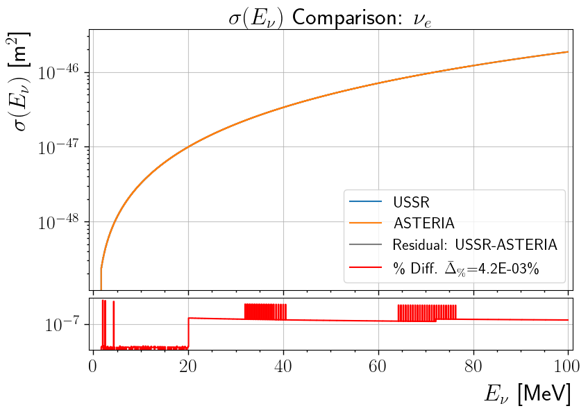
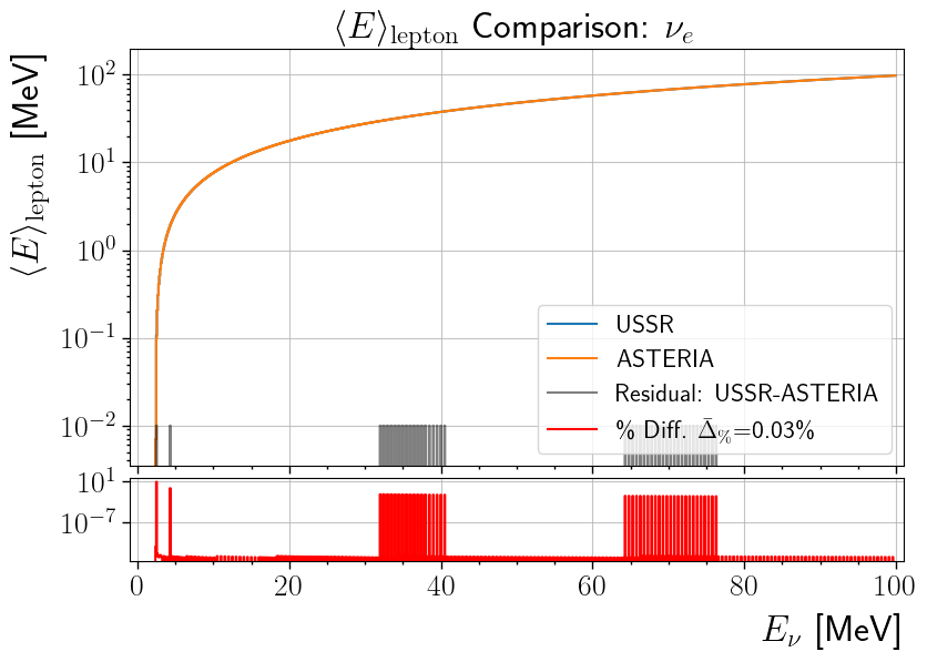
drawComparisonplots USSR’s reported values against ASTERIA’s reported values and computes the absolute difference and percent difference of ASTERIA’s reported value relative to USSR’s reported value. The average percent difference is denoted \(\bar{\Delta}_\%\). This average was taken over the entire curve excluding any points where USSR returned a value of 0.drawComparisonassumes that the two quantities being compared are plotted on the same domain, which is the case in this notebook.In other notebooks,
drawComparisonplots the raw difference, here it plots the absolute difference for the cross sections, so it may be plotted with the cross section on a semi-log plot.
getUSSRdataretrieves the specified file fromdata\USSR\. The array size is specified in the first line of the file’s header.getUSSRdataassumes that the data is sorted into columns such that the first is time in seconds, the next four columns are USSR’s reported cross sections for each flavor in the order \(\nu_e\), \(\bar{\nu}_e\), \(\nu_x\), \(\bar{\nu}_x\), and the next four are USSR’s reported mean lepton energies (in the same order). The files indata\USSR\were written accordingly.
[5]:
def drawComparison(t, ussr_y, astr_y, flavor, label='', units='', xs=False):
    # Compute difference and percent difference relative to USSR
    if xs:
        diff =  abs(ussr_y - astr_y)
    else:
        diff = ussr_y - astr_y
    pct_diff = 100*np.divide( abs(diff) , ussr_y,
                              where=ussr_y>0,
                              out=np.zeros_like(ussr_y) )

    # Compute average percent difference excluding where USSR Reported 0
    avg_pct_diff = np.mean( pct_diff[pct_diff>0] )

    fig, (ax1, ax2) = plt.subplots(2,1, figsize=(9,6),
                                   gridspec_kw = {'height_ratios':[5, 1]},
                                   sharex=True)

    # Plot USSR and ASTERIA against Each other.
    # Plot the abs difference between the two on the same figure.
    # Plot the percent difference on a subplot with a shared x-axis
    ax1.step( t, ussr_y, label='USSR')
    ax1.step( t, astr_y, label='ASTERIA')
    ax1.step( t, diff, 'k', label = 'Residual: USSR-ASTERIA', alpha=.50)
    if avg_pct_diff < 0.01:
        tmp_label = r'\% Diff. $\bar{\Delta}_\%$'+r'={0:6.1E}\%'.format(avg_pct_diff)
    else:
        tmp_label = r'\% Diff. $\bar{\Delta}_\%$'+r'={0:4.2f}\%'.format(avg_pct_diff)
    ax2.step( t, pct_diff, 'r', label = tmp_label)

    ttl = ax1.set_title( label+' Comparison: '+ flavor.to_tex() )
    # If this is a cross section plot, limit the y-axis and make it log-scaled.
    #  - This was done to make the cross sections easier to read, even though
    #    the graph of the residual is often cut off.
    if xs:
        ymin = np.min( np.append(ussr_y[ussr_y>0], astr_y[astr_y>0]) )
        ymax = np.max( np.append(ussr_y, astr_y) )
        ax1.set( ylim=(ymin/2, ymax*2), yscale='log' )
        ttl.set_position([.5, 1.025])

    ax1.set_ylabel( label+' '+units, horizontalalignment='right', y = 1)
    ax2.set( xlim=(-1, 101), yscale='log')
    ax2.set_xlabel(r'$E_\nu$ [MeV]', horizontalalignment='right', x = 1)


    # Group the labels of all lines in one legend object and display on axis 1
    handles, labels = ax1.get_legend_handles_labels()
    handles.append(ax2.get_legend_handles_labels()[0][0])
    labels.append(ax2.get_legend_handles_labels()[1][0])

    # Lock the legend to the lower right, In this notebook, this interferes with the
    #   graphs the least, despite differing with loc='best' for the legend.
    legend = ax1.legend( handles, labels, loc='lower right' )

    ax1.set_title( label+' Comparison: '+ flavor.to_tex() )

    # Return figure and axis handles for additional manipulation.
    return fig, (ax1, ax2)

def getUSSRdata(filename):
    fullpath = files('asteria.data').joinpath(f'USSR/{filename}')
    if not fullpath.exists():
        raise FileNotFoundError(f'{str(fullpath)} does not exist.')

    ussr = Table.read(fullpath,
                  format='ascii',
                  names=['Enu', 'xs_NU_E', 'xs_NU_E_BAR', 'xs_NU_X', 'xs_NU_X_BAR',
                                'Elep_NU_E', 'Elep_NU_E_BAR', 'Elep_NU_X', 'Elep_NU_X_BAR'])

    return ussr
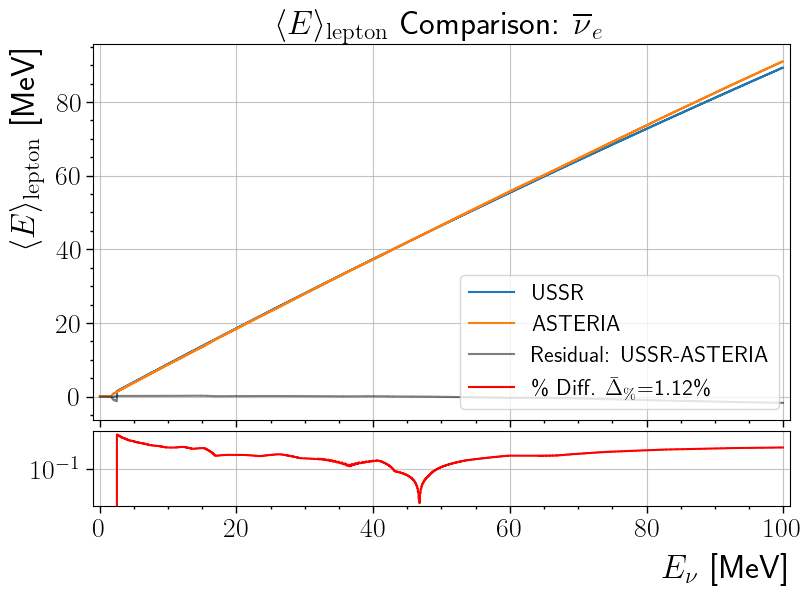
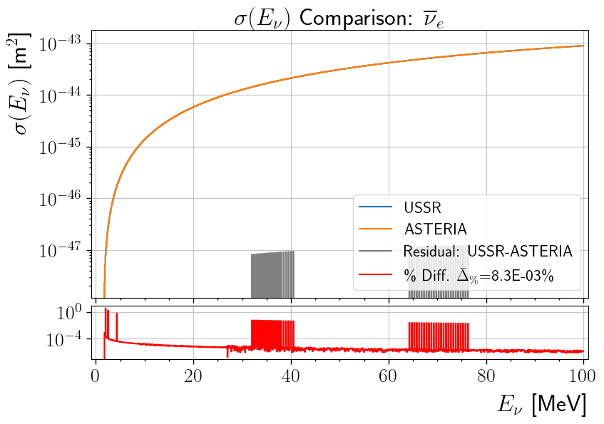
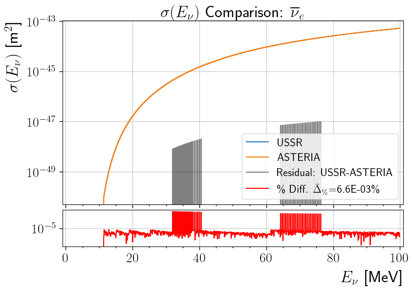
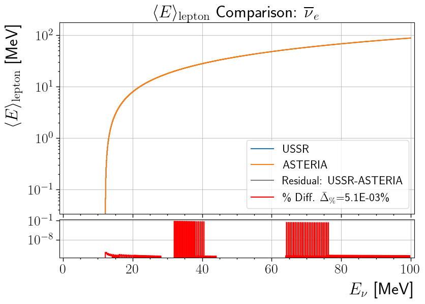
Plot Comparison of USSR’s IBD with ASTERIA’s Tabulated IBD
Only \(\bar{\nu}_e\) interact via IBD. This will compare the differential cross section and mean lepton energy reported by USSR with those reported by ASTERIA’s InvBetaTab(). This implementation differs with USSR more than InvBetaPar() as a table is interpolated rather than using a parameterization.
NOTE (03/13/19): It might be worth checking InvBetaTab() and comparing with Vissani Table 1 to make sure everything is correct.
[6]:
ussrdata = getUSSRdata('InvBeta.txt')
Enu = ussrdata['Enu']
interaction = interactions.InvBetaTab()

for nu, flavor in enumerate(Flavor):
    xsname = f'xs_{flavor.name}'
    ussrxs = ussrdata[xsname]
    astrxs = interaction.cross_section(flavor=flavor, e_nu=Enu*u.MeV).to_value('m**2')

    if astrxs.any() and ussrxs.any():
        drawComparison(Enu, ussrxs, astrxs, flavor, r'$\sigma(E_\nu)$',  '[m$^2$]', xs=True)

    mEname = f'Elep_{flavor.name}'
    ussrmE = ussrdata[mEname]
    astrmE = interaction.mean_lepton_energy(flavor=flavor, e_nu=Enu*u.MeV).to_value('MeV')

    if astrmE.any() and ussrmE.any():
        drawComparison(Enu, ussrmE, astrmE, flavor, r'$\langle E \rangle_\mathrm{lepton}$', '[MeV]')
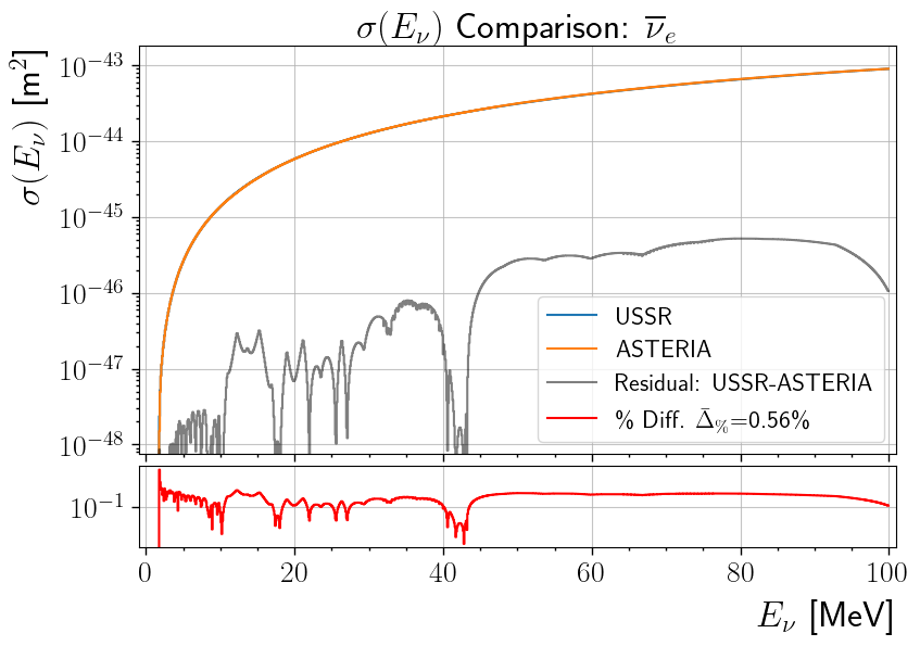
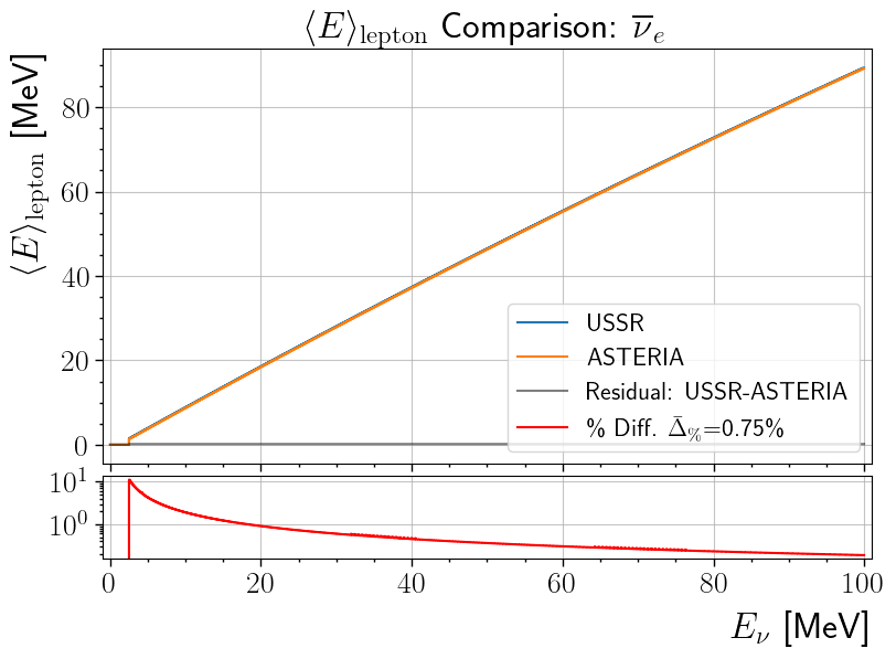
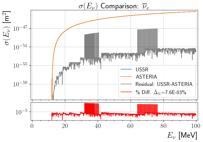
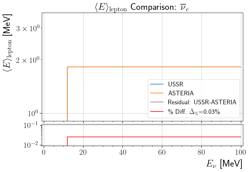
Plot Comparison of USSR’s IBD with ASTERIA’s Parameterized IBD
Only \(\bar{\nu}_e\) interact via IBD. This will compare the differential cross section and mean lepton energy reported by USSR with those reported by ASTERIA’s InvBetaPar(). This implementation is the same as USSR’s implementation.
[7]:
ussrdata = getUSSRdata('InvBeta.txt')
Enu = ussrdata['Enu']
interaction = interactions.InvBetaPar()

for nu, flavor in enumerate(Flavor):
    xsname = f'xs_{flavor.name}'
    ussrxs = ussrdata[xsname]
    astrxs = interaction.cross_section(flavor=flavor, e_nu=Enu*u.MeV).to_value('m**2')

    if astrxs.any() and ussrxs.any():
        drawComparison(Enu, ussrxs, astrxs, flavor, r'$\sigma(E_\nu)$',  '[m$^2$]', xs=True)

    mEname = f'Elep_{flavor.name}'
    ussrmE = ussrdata[mEname]
    astrmE = interaction.mean_lepton_energy(flavor=flavor, e_nu=Enu*u.MeV).to_value('MeV')

    if astrmE.any() and ussrmE.any():
        drawComparison(Enu, ussrmE, astrmE, flavor, r'$\langle E \rangle_\mathrm{lepton}$', '[MeV]')
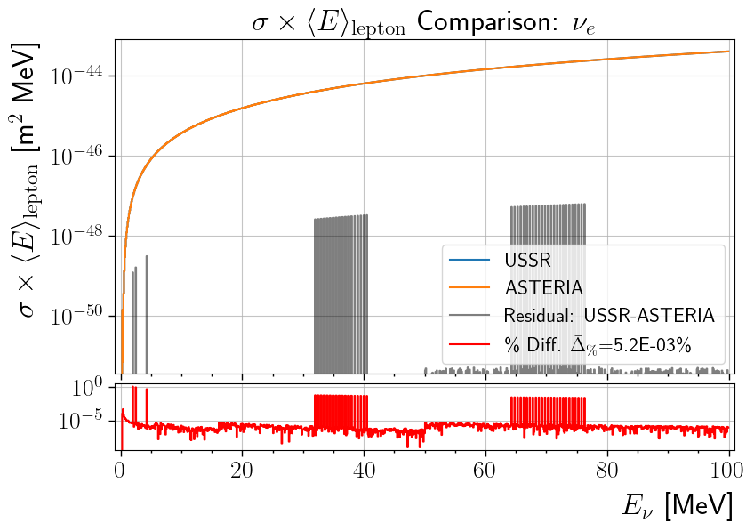
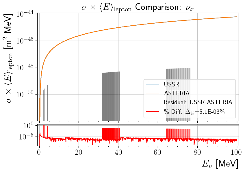
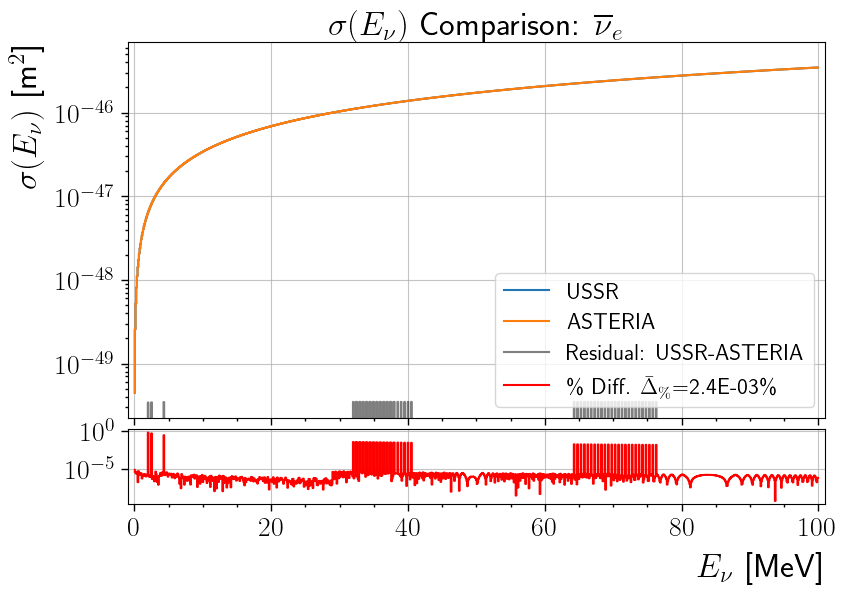
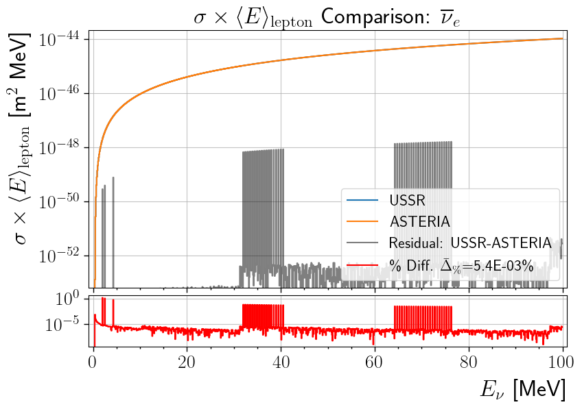
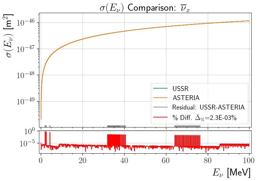
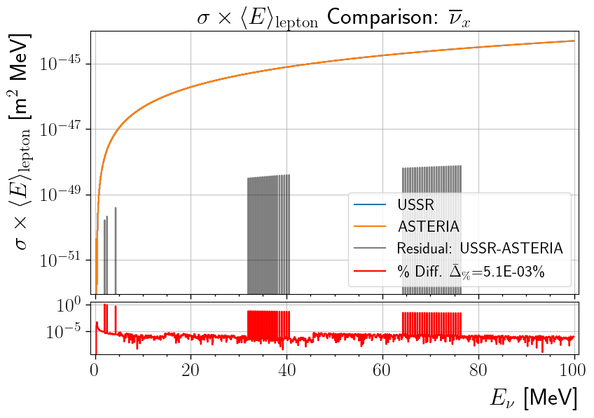
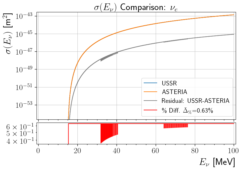
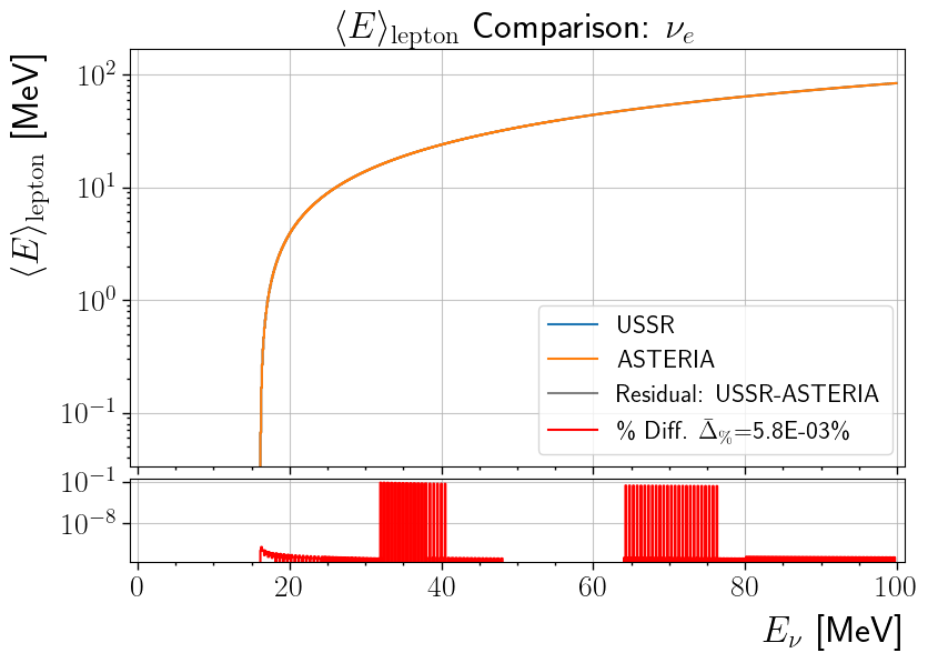
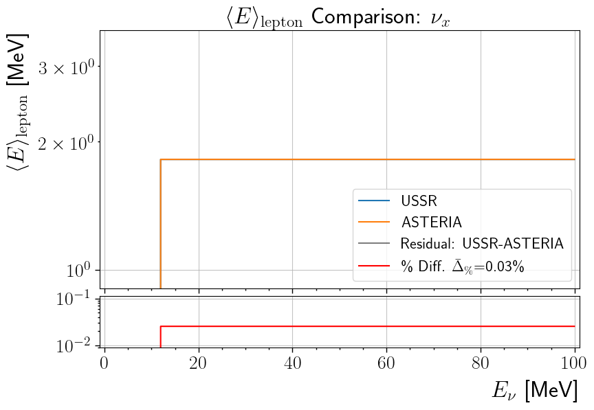
Plot Electron Scattering Comparisons for Each Flavor
All Flavors interact via Electron Scattering. This will compare each flavor’s differential cross section and mean energy as it is reported by ASTERIA and USSR. In this case, the mean lepton energy that is reported is the product of the differential cross section with the lepton energy, integrated w.r.t lepton energy, It has units m\(^2\) MeV.
NOTE (03/13/19): I have thought about changing the implementation of ElectronScatter()’s mean energy to return a quantity with units MeV. That is, take the integrated product we have now, and divide it by the differential cross section. This is NOT how USSR implements it, and at the time of writing ASTERIA does NOT do this.
NOTE (04/22/19): I have implemented the change made in my previous comment. Taking a slight hit to performance, the ElectronScatter.mean_lepton_energy method now returns units \(MeV\). This is a achieved by dividing the previous result by the cross section.
[8]:
astrmE = interactions.ElectronScatter().mean_lepton_energy(flavor=Flavor.NU_E, e_nu=Enu*u.MeV).to_value('MeV')
ussrdata
[8]:
| Enu | xs_NU_E | xs_NU_E_BAR | xs_NU_X | xs_NU_X_BAR | Elep_NU_E | Elep_NU_E_BAR | Elep_NU_X | Elep_NU_X_BAR |
|---|---|---|---|---|---|---|---|---|
| float64 | float64 | float64 | float64 | float64 | float64 | float64 | float64 | float64 |
| 0.05 | 0.0 | 0.0 | 0.0 | 0.0 | 0.0 | 0.0 | 0.0 | 0.0 |
| 0.15 | 0.0 | 0.0 | 0.0 | 0.0 | 0.0 | 0.0 | 0.0 | 0.0 |
| 0.25 | 0.0 | 0.0 | 0.0 | 0.0 | 0.0 | 0.0 | 0.0 | 0.0 |
| 0.35 | 0.0 | 0.0 | 0.0 | 0.0 | 0.0 | 0.0 | 0.0 | 0.0 |
| 0.45 | 0.0 | 0.0 | 0.0 | 0.0 | 0.0 | 0.0 | 0.0 | 0.0 |
| 0.55 | 0.0 | 0.0 | 0.0 | 0.0 | 0.0 | 0.0 | 0.0 | 0.0 |
| 0.65 | 0.0 | 0.0 | 0.0 | 0.0 | 0.0 | 0.0 | 0.0 | 0.0 |
| 0.75 | 0.0 | 0.0 | 0.0 | 0.0 | 0.0 | 0.0 | 0.0 | 0.0 |
| 0.85 | 0.0 | 0.0 | 0.0 | 0.0 | 0.0 | 0.0 | 0.0 | 0.0 |
| ... | ... | ... | ... | ... | ... | ... | ... | ... |
| 99.05 | 0.0 | 8.8564467e-44 | 0.0 | 0.0 | 0.0 | 88.589774 | 0.0 | 0.0 |
| 99.15 | 0.0 | 8.8688145e-44 | 0.0 | 0.0 | 0.0 | 88.671694 | 0.0 | 0.0 |
| 99.25 | 0.0 | 8.8811827e-44 | 0.0 | 0.0 | 0.0 | 88.753597 | 0.0 | 0.0 |
| 99.35 | 0.0 | 8.8935514e-44 | 0.0 | 0.0 | 0.0 | 88.835485 | 0.0 | 0.0 |
| 99.45 | 0.0 | 8.9059205e-44 | 0.0 | 0.0 | 0.0 | 88.917357 | 0.0 | 0.0 |
| 99.55 | 0.0 | 8.91829e-44 | 0.0 | 0.0 | 0.0 | 88.999214 | 0.0 | 0.0 |
| 99.65 | 0.0 | 8.9306598e-44 | 0.0 | 0.0 | 0.0 | 89.081054 | 0.0 | 0.0 |
| 99.75 | 0.0 | 8.9430301e-44 | 0.0 | 0.0 | 0.0 | 89.162879 | 0.0 | 0.0 |
| 99.85 | 0.0 | 8.9554007e-44 | 0.0 | 0.0 | 0.0 | 89.244688 | 0.0 | 0.0 |
| 99.95 | 0.0 | 8.9677717e-44 | 0.0 | 0.0 | 0.0 | 89.326481 | 0.0 | 0.0 |
[9]:
ussrdata = getUSSRdata('ElectronScatter.txt')
Enu = ussrdata['Enu']
interaction = interactions.ElectronScatter()

for nu, flavor in enumerate(Flavor):
    xsname = f'xs_{flavor.name}'
    ussrxs = ussrdata[xsname]
    astrxs = interaction.cross_section(flavor=flavor, e_nu=Enu*u.MeV).to_value('m**2')

    if astrxs.any() and ussrxs.any():
        drawComparison(Enu, ussrxs, astrxs, flavor, r'$\sigma(E_\nu)$',  '[m$^2$]', xs=True)

    mEname = f'Elep_{flavor.name}'
    ussrmE = ussrdata[mEname]
    astrmE = interaction.mean_lepton_energy(flavor=flavor, e_nu=Enu*u.MeV).to_value('MeV') * astrxs

    if astrmE.any() and ussrmE.any():
        drawComparison(Enu, ussrmE, astrmE, flavor, r'$\sigma \times \langle E \rangle_\mathrm{lepton}$', '[m$^2$ MeV]', xs=True)
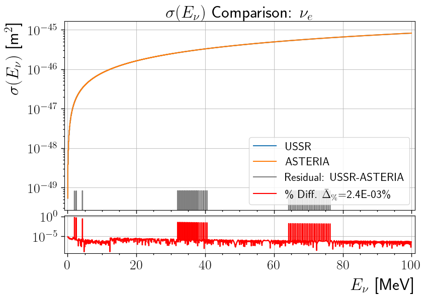

Plot Oxygen-16 Charged Current Comparisons for \(\nu_e\) and \(\bar{\nu}_e\)
Only \(\nu_e\) and \(\bar{\nu}_e\) interact via charged currents with Oxygen-16. This will compare each flavor’s differential cross section and mean energy as it is reported by ASTERIA and USSR.
[10]:
ussrdata = getUSSRdata('Oxygen16CC.txt')
Enu = ussrdata['Enu']
interaction = interactions.Oxygen16CC()

for nu, flavor in enumerate(Flavor):
    xsname = f'xs_{flavor.name}'
    ussrxs = ussrdata[xsname]
    astrxs = interaction.cross_section(flavor=flavor, e_nu=Enu*u.MeV).to_value('m**2')

    if astrxs.any() and ussrxs.any():
        drawComparison(Enu, ussrxs, astrxs, flavor, r'$\sigma(E_\nu)$',  '[m$^2$]', xs=True)

    mEname = f'Elep_{flavor.name}'
    ussrmE = ussrdata[mEname]
    astrmE = interaction.mean_lepton_energy(flavor=flavor, e_nu=Enu*u.MeV).to_value('MeV')

    if astrmE.any() and ussrmE.any():
        drawComparison(Enu, ussrmE, astrmE, flavor, r'$\langle E \rangle_\mathrm{lepton}$', '[MeV]', xs=True)
Plot Oxygen-16 Neutral Current Comparisons for Each Flavor
All Flavors interact via neutral currents with Oxygen-16. This will compare each flavor’s differential cross section and mean energy as it is reported by ASTERIA and USSR.
[11]:
ussrdata = getUSSRdata('Oxygen16NC.txt')
Enu = ussrdata['Enu']
interaction = interactions.Oxygen16NC()

for nu, flavor in enumerate(Flavor):
    xsname = f'xs_{flavor.name}'
    ussrxs = ussrdata[xsname]
    astrxs = interaction.cross_section(flavor=flavor, e_nu=Enu*u.MeV).to_value('m**2')

    if astrxs.any() and ussrxs.any():
        drawComparison(Enu, ussrxs, astrxs, flavor, r'$\sigma(E_\nu)$',  '[m$^2$]', xs=True)

    mEname = f'Elep_{flavor.name}'
    ussrmE = ussrdata[mEname]
    astrmE = interaction.mean_lepton_energy(flavor=flavor, e_nu=Enu*u.MeV).to_value('MeV')

    if astrmE.any() and ussrmE.any():
        drawComparison(Enu, ussrmE, astrmE, flavor, r'$\langle E \rangle_\mathrm{lepton}$', '[MeV]', xs=True)


Plot Oxygen-18 Charged Current Comparisons for \(\nu_e\).
Only \(\nu_e\) interact via charged currents with Oxygen-18. This will compare each flavor’s differential cross section and mean energy as it is reported by ASTERIA and USSR.
NOTE (03/13/19): This parameterization was obtained using a quadratic fit to cross section estimated from Kamiokande data from Haxton and Robertson, PRC 59:515, 1999. See also, the page on the Mainz Wiki, Neutrino cross sections on natural oxygen. The cross section includes one additional scaling factor of one over the abundance of O\(^{18}\), and it is unclear why this is present. It would make more sense if the cross sectin was scaled by the oxygen abundance. This scaling factor currently features both in USSR and ASTERIA.
[12]:
ussrdata = getUSSRdata('Oxygen18.txt')
Enu = ussrdata['Enu']
interaction = interactions.Oxygen18()

for nu, flavor in enumerate(Flavor):
    xsname = f'xs_{flavor.name}'
    ussrxs = ussrdata[xsname]
    astrxs = interaction.cross_section(flavor=flavor, e_nu=Enu*u.MeV).to_value('m**2')

    if astrxs.any() and ussrxs.any():
        drawComparison(Enu, ussrxs, astrxs, flavor, r'$\sigma(E_\nu)$',  '[m$^2$]', xs=True)

    mEname = f'Elep_{flavor.name}'
    ussrmE = ussrdata[mEname]
    astrmE = interaction.mean_lepton_energy(flavor=flavor, e_nu=Enu*u.MeV).to_value('MeV')

    if astrmE.any() and ussrmE.any():
        drawComparison(Enu, ussrmE, astrmE, flavor, r'$\langle E \rangle_\mathrm{lepton}$', '[MeV]', xs=True)