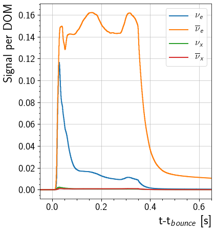
Signal per DOM

Load a simulation and plot the signal per DOM.

[1]:

from asteria import config, source, IO
from asteria.interactions import Interactions
from asteria.neutrino import Flavor
from asteria.config import parse_quantity
import astropy.units as u

import numpy as np
import matplotlib as mpl
import matplotlib.pyplot as plt

Set up styles for plotting

[2]:

axes_style =   {            'grid' : 'True',
                       'labelsize' : '24',
                        'labelpad' : '8.0' }

xtick_style =  {       'direction' : 'out',
                       'labelsize' : '20.',
                      'major.size' : '5.',
                     'major.width' : '1.',
                   'minor.visible' : 'True',
                      'minor.size' : '2.5',
                     'minor.width' : '1.' }

ytick_style =  {       'direction' : 'out',
                       'labelsize' : '20.',
                      'major.size' : '5',
                     'major.width' : '1.',
                   'minor.visible' : 'True',
                      'minor.size' : '2.5',
                     'minor.width' : '1.' }

grid_style =   {           'alpha' : '0.75' }
legend_style = {        'fontsize' : '18' }
font_syle =    {            'size' : '20'}
text_style =   {          'usetex' : 'True' }
figure_style = {  'subplot.hspace' : '0.05' }

mpl.rc(    'font', **font_syle )
mpl.rc(    'text', **text_style )
mpl.rc(    'axes', **axes_style )
mpl.rc(   'xtick', **xtick_style )
mpl.rc(   'ytick', **ytick_style )
mpl.rc(    'grid', **grid_style )
mpl.rc(  'legend', **legend_style )
mpl.rc(  'figure', **figure_style )

mpl.rcParams['text.usetex'] = True
mpl.rcParams['text.latex.preamble'] = [r'\usepackage[cm]{sfmath}']

Load Configuration

This will load the source configuration from a file.

For this to work, either the user needs to have done one of two things:

Run python setup.py install in the ASTERIA directory.
Run python setup.py develop and set the environment variable ASTERIA to point to the git source checkout.

If these were not done, the initialization will fail because the paths will not be correctly resolved.

[3]:

conf = config.load_config('../../data/config/default.yaml')
ccsn = source.initialize(conf)

Prepare Iterables

Read from the configuration, the range of neutrino energies (Enu) to simulate and the times (time) at which to perform the simulation. Defining the time and energy arrays in this manner (end-point inclusive) aligns with the definition in asteria.simulationHandler.

[4]:

# Define neutrino energy spectrum
E_min = parse_quantity(conf.simulation.energy.min).to(u.MeV).value
E_max = parse_quantity(conf.simulation.energy.max).to(u.MeV).value
dE = parse_quantity(conf.simulation.energy.step).to(u.MeV).value
Enu = np.arange(E_min, E_max+dE, dE) * u.MeV

# Define post-bounce times at which to evaluate
t_min = parse_quantity(conf.simulation.time.min).to(u.s).value
t_max = parse_quantity(conf.simulation.time.max).to(u.s).value
dt = parse_quantity(conf.simulation.time.step).to(u.s).value
time = np.arange(t_min, t_max+dt, dt) * u.s

Load Simulation and Compute Signal per DOM

Import a simulation from the file \data\processed\nakazato-shen-z0.02-t_rev300ms-s13.0.h5 using IO.load(). It is assumed that this file has already been generated\(^*\). This file is specific to the model and its path is stored in the conf object. The configuration parameters describing the simulation are contained within the config.simulation node as follows…

interactions The neutrino interactions used to perform the simulation
flavors The neutrino flavors used to perform the simulation
hierarchy The neutrino mass hierarchy used to perform neutrino oscillations.
energy The Energy resolution at which cross sections, lepton mean energy, and the source PDFs were binned.
- Contains 4 nodes min, max, step, and size
time The Time resolution at which the simulation profile is binned.
- Contains 4 nodes min, max, step, and size

If no object is found, None will be returned.

The code to save a simulation to file is …

IO.save(conf, result)

Where result is the photonic energy deposition in 1 m\(^3\) of ice scaled to a progenitor that is 1 kpc away. This is scaled to progenitor distance of the source and the effective volume of a DOM to find the expected signal increase for a single DOM.

\(^*\)NOTE: This notebook assumes that the simulation described in \data\config\default.yaml has already been performed and saved. It will be written to the file \data\processed\nakazato-shen-z0.02-t_rev300ms-s13.0.h5. To generate this file, run the notebook \docs\nb\detector_response.ipynb.

[5]:

effvol = 0.1654 * u.m**3 / u.MeV

E_per_V = IO.load(conf) * u.MeV / u.m**3
E_per_V /= ccsn.progenitor_distance.to(u.kpc).value**2
signal_per_DOM = effvol * E_per_V

Plot Signal Increase Per DOM

This will plot the signal increase in a single DOM caused by each flavor. The curve shows the DOM response from 0.05 seconds before the core bounce to 0.65 seconds after the core bounce. Note that this is computed with the assumption that the effective volume of the DOM is 0.1654 m\(^3\) MeV\(^{-1}\)

[6]:

fig, ax = plt.subplots(1, figsize = (6,7))

for nu, flavor in enumerate(Flavor):
    ax.step( time, signal_per_DOM[nu], label=flavor.to_tex(), linewidth=2)

ax.set_ylabel( 'Signal per DOM', horizontalalignment='right', y = 1)
ax.set_xlabel(r't-t$_{bounce}$ [s]', horizontalalignment='right', x=1.0)
ax.set(xlim=(-0.05, 0.65))
ax.legend()

[6]:

<matplotlib.legend.Legend at 0x7fb4f14ee550>

[ ]: