Create ROOT File from ASTERIA Simulation
[1]:
from astropy.utils.exceptions import AstropyDeprecationWarning
from asteria import set_rcparams
from asteria.simulation import Simulation
from snewpy.neutrino import Flavor

import matplotlib.pyplot as plt
import astropy.units as u

import numpy as np
import uproot
import os
import warnings
warnings.simplefilter(action='ignore', category=(FutureWarning, AstropyDeprecationWarning))
/home/docs/checkouts/readthedocs.org/user_builds/asteria/envs/latest/lib/python3.12/site-packages/tqdm/auto.py:21: TqdmWarning: IProgress not found. Please update jupyter and ipywidgets. See https://ipywidgets.readthedocs.io/en/stable/user_install.html
  from .autonotebook import tqdm as notebook_tqdm
Set up Plotting Defaults
[2]:
set_rcparams()
Set up and Run a Model
[3]:
model = {
'name': 'Sukhbold_2015',
'param':{
'progenitor_mass': 27*u.Msun,
'eos': 'LS220'}
}
Emin=0*u.MeV; Emax=100*u.MeV; dE=1*u.MeV
tmin=-1*u.s; tmax=10*u.s; dt=2*u.ms
params = {
'model': model,
'distance':1*u.kpc,
'Emin':0*u.MeV, 'Emax':100*u.MeV, 'dE':1*u.MeV,
'tmin':-1*u.s, 'tmax':10*u.s, 'dt':2*u.ms,
'mixing_scheme':'AdiabaticMSW',
'hierarchy':'normal'
}
sim = Simulation(**params)
sim.run()
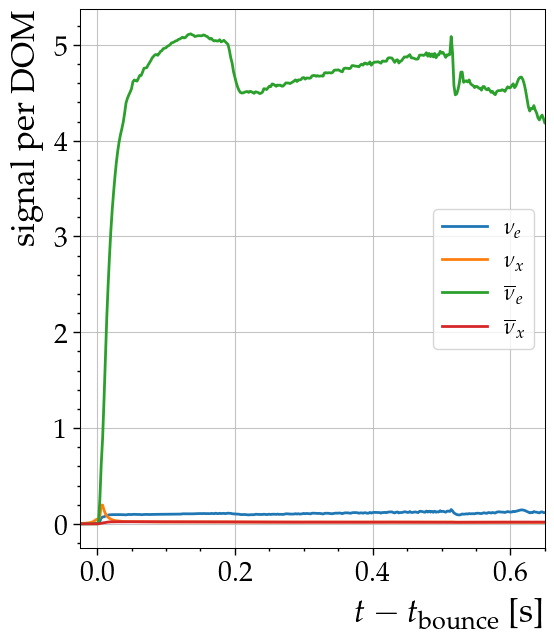
time = np.append(sim.time, sim.time[-1] + sim._sim_dt)
fig, ax = plt.subplots(1, figsize = (6,7))
for flavor in sim.flavors:
ax.plot(sim.time, sim.avg_dom_signal(flavor=flavor), label=flavor.to_tex())
ax.legend()
ax.set(xlabel=r'$t-t_\mathrm{bounce}$ [s]', ylabel='signal per DOM', xlim=(-0.025, 0.65));
sukhbold-LS220-s27.0.fits: 100%|██████████| 782k/782k [00:00<00:00, 207MiB/s]
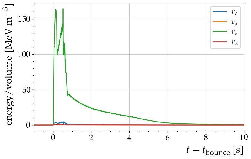
[4]:
fig, ax = plt.subplots(1, figsize=(9,5.5))

for flavor in Flavor:
    ax.plot(sim.time, sim.E_per_V[flavor], label=flavor.to_tex())
ax.set(xlabel=r'$t-t_\mathrm{bounce}$ [s]',
       xlim=(sim.time[0].to_value('s'), sim.time[-1].to_value('s')),
       ylabel=r'energy/volume [MeV m$^{-3}$]')
ax.legend();
Create ROOT file
Create np.histogram, using the simulation time binning and total signal per DOM. Create ROOT file using histogram.
[5]:
outfile = 'Sukhbold_s27_LS220.root'
with uproot.recreate(outfile) as file:
    file['total_photonic_energy_distance_1kpc'] = np.histogram(sim.time.value, bins=time.value, weights=sim.total_E_per_V.value)
    file['version'] = '1.2'
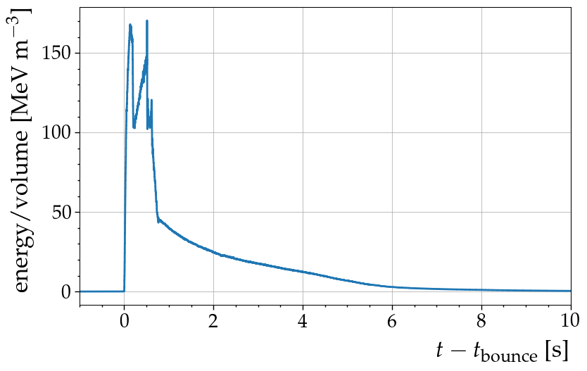
[6]:
variable = np.histogram(sim.time.value, bins=time.value, weights=sim.total_E_per_V.value)

fig, ax = plt.subplots(1, figsize=(9,5.5))
ax.step(variable[1][:-1], variable[0])
ax.set(xlabel=r'$t-t_\mathrm{bounce}$ [s]',
       xlim=(sim.time[0].to_value('s'), sim.time[-1].to_value('s')),
       ylabel=r'energy/volume [MeV m$^{-3}$]');