Detector Hits + Oscillations 1 (Obsolete)

Demonstrate the total number of hits in the IceCube detector after implementaing neutrino oscillations.

This notebook uses files generated using the notebook detector_hits_file.

The progenitor model used is the Nakazato Shen model with z = 0.02, t\(_{rev}\) = 300ms, m = 13.0M\(_\odot\)

from astropy import units as u
from astropy.table import Table

import numpy as np
import matplotlib as mpl
import matplotlib.pyplot as plt

from asteria import config, source, detector
from asteria.neutrino import Flavor

mpl.rc('font', size=18)

Prepare Iterables

Define the range of neutrino energies (E_nu) to simulate and the times (time) and distances (dist) at which to perform the simulation. The progenitor distance is set to 1 kpc.

E_min = 0.1; E_max = 100.1; dE = 0.1;
Enu = np.arange(E_min, E_max, dE) * u.MeV

t_min = -1; t_max = 15; dt = 0.0001;
time = np.arange(t_min, t_max, dt) * u.s

Load Configuration

This will load the source configuration from a file.

For this to work, either the user needs to have done one of two things:

1. Run python setup.py install in the ASTERIA directory.

2. Run python setup.py develop and set the environment variable ASTERIA to point to the git source checkout.

If these were not done, the initialization will fail because the paths will not be correctly resolved.

conf = config.load_config('../../data/config/nakazato-shen-z0.02-t_rev300ms-s13.0.yaml')
ccsn = source.initialize(conf)
ic86 = detector.initialize(conf)

icecube_dt = 2e-3 #s
deadtime = 0.25e-3
dc_rel_eff = 1.35

doms = ic86.doms_table()
n_i3_doms = len(doms[doms['type'] == 'i3'])
n_dc_doms = len(doms[doms['type'] == 'dc'])

i3_dom_bg_mu = 284.9
i3_dom_bg_sig = 26.2

dc_dom_bg_mu = 358.9;
dc_dom_bg_sig = 36.0;

i3_bg_mu  = 2933.72
i3_bg_sig = 85.8662

Define Helper Functions

• hits Scale the original signal signal calculated for a progenitor at 1 kpc by the distance dist of the new progenitor, and use the new signal to generate and return detector hits for the given progenitor. The deadtime fractions used to generate hits are scaled by the timebin being used.

• rebin Reshape the independent variable var with resolution old_binning and dependent variable data (assumed to be numpy array) and return new arrays var and data with resolution new_binning.

• background Use timebin to scale the mean background and the uncertainty, and return a randomly sampled array of length len_array.

def hits(signal, dist, timebin):
    total_signal = np.sum(signal, axis = 0) / dist**2
    eps_i3 = 0.87 / (1+deadtime* total_signal/timebin)
    eps_dc = 0.87 / (1+deadtime*total_signal*dc_rel_eff/timebin)
    hits = ic86.detector_hits(abs(total_signal), eps_i3, eps_dc)
    return hits

def rebin(var, data, old_binning, new_binning):
    step = int(new_binning/old_binning)
    new_size = int(data.size / step)

    rebinned_data = np.sum(np.split( data, new_size ), axis=1)
    rebinned_var  = var.value[int(0.5 * step)::step]

    return rebinned_var, rebinned_data

def background(timebin, len_array):
    # Calculating Background:
    dr  = (n_i3_doms*i3_dom_bg_mu + n_dc_doms*dc_dom_bg_mu ) * timebin;
    dr_er = np.sqrt((n_i3_doms*i3_dom_bg_sig**2 + n_dc_doms*dc_dom_bg_sig**2) * timebin)
    return np.random.normal(dr, dr_er, len_array)

Read Data from nakazato-shen-z0.02-t_rev300ms-s13.0_e_per_v.fits

table = Table.read('nakazato-shen-z0.02-t_rev300ms-s13.0_e_per_v.fits')

sig = np.asarray([table['unmixed nu_e sig'], table['unmixed nu_e_bar sig'], table['unmixed nu_x sig'], table['unmixed nu_x_bar sig']])
sig_norm = np.asarray([table['normal nu_e sig'], table['normal nu_e_bar sig'], table['normal nu_x sig'], table['normal nu_x_bar sig']])
sig_inv = np.asarray([table['inverted nu_e sig'], table['inverted nu_e_bar sig'], table['inverted nu_x sig'], table['inverted nu_x_bar sig']])

# Scale signal to icecube_dt
sig_2ms = []
sig_norm_2ms = []
sig_inv_2ms = []
for i in range(len(Flavor)):
    time_2ms, sig_ = rebin(time, sig[i], dt, icecube_dt)
    time_2ms, sig_norm_ = rebin(time, sig_norm[i], dt, icecube_dt)
    time_2ms, sig_inv_ = rebin(time, sig_inv[i], dt, icecube_dt)
    sig_2ms.append(sig_)
    sig_norm_2ms.append(sig_norm_)
    sig_inv_2ms.append(sig_inv_)

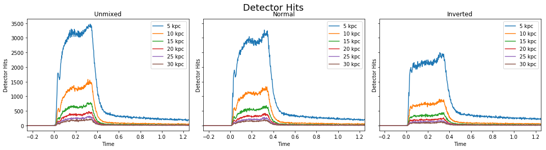
Generate Plots

Hits vs time for various progenitor distances

## Plotting nu_e_bar hits for each oscillation scenario
fig, axes = plt.subplots(1, 3, figsize = (15, 4), sharex = True, sharey = True)
ax1, ax2, ax3 = axes
fig.suptitle(r'Detector Hits', fontsize = 18, y = 1.015)
for d in range(5, 31, 5):
    new_hits = hits(sig_2ms, d, icecube_dt)
    hits_n = hits(sig_norm_2ms, d, icecube_dt)
    hits_i = hits(sig_inv_2ms, d, icecube_dt)

    ax1.plot(time_2ms, new_hits, label = '{0} kpc'.format(d))
    ax1.set(#xlim = (0, 0.1),
           xlabel = 'Time',
           ylabel = 'Detector Hits',
           title = 'Unmixed')
    ax1.legend()

    ax2.plot(time_2ms, hits_n, label = '{0} kpc'.format(d))
    ax2.set(xlim = (-0.25, 1.25),
           xlabel = 'Time',
           ylabel = 'Detector Hits',
           title = 'Normal')
    ax2.legend()

    ax3.plot(time_2ms, hits_i, label = '{0} kpc'.format(d))
    ax3.set(#xlim = (-0.25, 1.25),
           xlabel = 'Time',
           ylabel = 'Detector Hits',
           title = 'Inverted')
    ax3.legend()

fig.tight_layout()
# fig.subplots_adjust(top = 0.88)

Hits + Backgroud for 10kpc

fig, axes = plt.subplots(1, 3, figsize = (15, 4), sharex = True, sharey = True)
ax1, ax2, ax3 = axes
fig.suptitle(r'Detector Hits + BG, 10kpc', fontsize = 18, y = 1.017)
new_hits = hits(sig_2ms, 10, icecube_dt)
hits_n = hits(sig_norm_2ms, 10, icecube_dt)
hits_i = hits(sig_inv_2ms, 10, icecube_dt)

ax1.plot(time_2ms, new_hits + background(icecube_dt, len(time_2ms)))
ax1.set(#xlim = (0, 0.1),
       xlabel = 'Time',
       ylabel = 'Detector Hits',
       title = 'Unmixed')

ax2.plot(time_2ms, hits_n + background(icecube_dt, len(time_2ms)))
ax2.set(#xlim = (-0.25, 1.25),
       xlabel = 'Time',
       ylabel = 'Detector Hits',
       title = 'Normal')

ax3.plot(time_2ms, hits_i + background(icecube_dt, len(time_2ms)))
ax3.set(#xlim = (-0.25, 1.25),
       xlabel = 'Time',
       ylabel = 'Detector Hits',
       title = 'Inverted')

fig.tight_layout()
# fig.subplots_adjust(top = 0.88)