Detector Hits in IceCube-Gen2

Demonstrate detector hits in the IC86 + Gen2 configuration of IceCube.

This includes both mDOMs and WLS modules.

from astropy import units as u

import numpy as np
import matplotlib as mpl
import matplotlib.pyplot as plt

from snewpy.neutrino import Flavor

from asteria.simulation import Simulation
from asteria import set_rcparams
from asteria import interactions

from importlib.resources import files

set_rcparams(verbose=False)

/home/docs/checkouts/readthedocs.org/user_builds/asteria/envs/latest/lib/python3.12/site-packages/tqdm/auto.py:21: TqdmWarning: IProgress not found. Please update jupyter and ipywidgets. See https://ipywidgets.readthedocs.io/en/stable/user_install.html
  from .autonotebook import tqdm as notebook_tqdm

Configure an mDOM Gen2 Simulation

Set up a progenitor 10 kpc from Earth and generate simulated hits.

To simulate the Gen2 detector, add the argument detector_scope='Gen2' when initializing the simulation.

model = {'name': 'Nakazato_2013',
         'param':{
             'progenitor_mass': 13 * u.Msun,
             'revival_time': 300 * u.ms,
             'metallicity': 0.004,
             'eos': 'shen'}
         }

sim = Simulation(model=model,
                 distance=10 * u.kpc,
                 Emin=0*u.MeV, Emax=100*u.MeV, dE=1*u.MeV,
                 tmin=-1*u.s, tmax=1*u.s, dt=1*u.ms,
                 detector_scope='Gen2')
sim.run()

nakazato-shen-z0.004-t_rev300ms-s13.0.fits: 100%|██████████| 36.6k/36.6k [00:00<00:00, 60.0MiB/s]

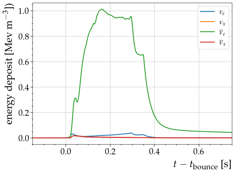
Plot the Energy Deposit

fig, ax = plt.subplots(1,1, figsize=(8,6), tight_layout=True)

for flavor in sim.flavors:
    ax.plot(sim.time, sim.E_per_V[flavor], label=flavor.to_tex())
ax.legend()
ax.set(xlabel=r'$t-t_\mathrm{bounce}$ [s]',
       ylabel='energy deposit [Mev m$^{-3}$])',
       xlim=(-0.15, 0.75));

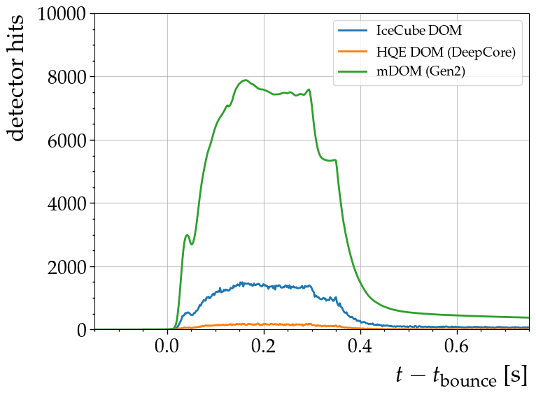
Plot Detector Response

Expected Signal from Each Subdetector

Set a time resolution dt. Using the sim.detector_signal() function we can read out the detector signal for each subdetector class. Separately plot hits from the main IceCube strings and DeepCore.

dt = 2 * u.ms
t, sim_i3 = sim.detector_signal(subdetector='i3', dt=dt)
t, sim_dc = sim.detector_signal(subdetector='dc', dt=dt)
t, sim_md = sim.detector_signal(subdetector='md', dt=dt)

fig, ax = plt.subplots(1,1, figsize=(8,6), tight_layout=True)
ax.plot(t, sim_i3, label='IceCube DOM')
ax.plot(t, sim_dc, label='HQE DOM (DeepCore)')
ax.plot(t, sim_md, label='mDOM (Gen2)')
ax.legend(fontsize=14)
ax.set(xlabel=r'$t-t_\mathrm{bounce}$ [s]',
       ylabel=f'detector hits',
       xlim=(-0.15, 0.75),
       ylim=(0,10000));

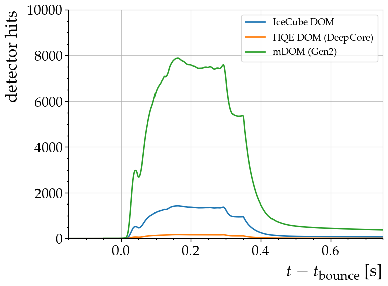
Generated Hits from Signal Only

t, hits_i3 = sim.detector_hits(subdetector='i3', dt=dt)
t, hits_dc = sim.detector_hits(subdetector='dc', dt=dt)
t, hits_md = sim.detector_signal(subdetector='md', dt=dt)

fig, ax = plt.subplots(1,1, figsize=(8,6), tight_layout=True)
ax.plot(t, hits_i3, label='IceCube DOM')
ax.plot(t, hits_dc, label='HQE DOM (DeepCore)')
ax.plot(t, hits_md, label='mDOM (Gen2)')

ax.legend(fontsize=14)
ax.set(xlabel=r'$t-t_\mathrm{bounce}$ [s]',
       ylabel=f'detector hits',
       xlim=(-0.15, 0.75),
       ylim=(0,10000));

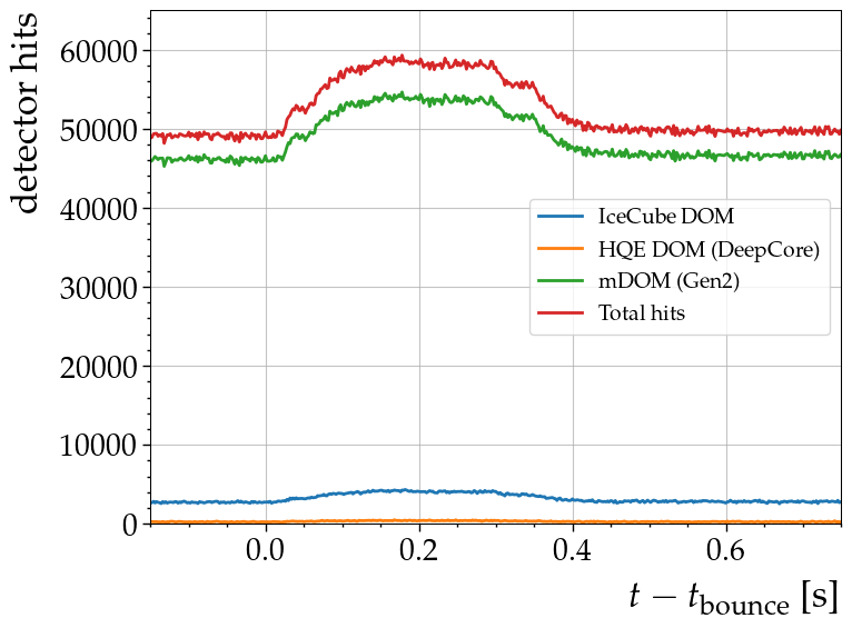
Generated Hits from Signal + Background

Separately compute the background hits and signal from each subdetector and add them.

bkg_i3 = sim.detector.i3_bg(dt, size=hits_i3.size)
bkg_dc = sim.detector.dc_bg(dt, size=hits_dc.size)
bkg_md = sim.detector.md_bg(dt, size=hits_md.size)

bkg = bkg_i3 + bkg_dc + bkg_md
hits = hits_i3 + hits_dc + hits_md

fig, ax = plt.subplots(1,1, figsize=(8,6), tight_layout=True)
ax.plot(t, hits_i3 + bkg_i3, label='IceCube DOM')
ax.plot(t, hits_dc + bkg_dc, label='HQE DOM (DeepCore)')
ax.plot(t, hits_md + bkg_md, label='mDOM (Gen2)')
ax.plot(t, hits + bkg, label='Total hits')

ax.legend(loc='center right', fontsize=14)
ax.set(xlabel=r'$t-t_\mathrm{bounce}$ [s]',
       ylabel=f'detector hits',
       xlim=(-0.15, 0.75),
       ylim=(0,65000)
);

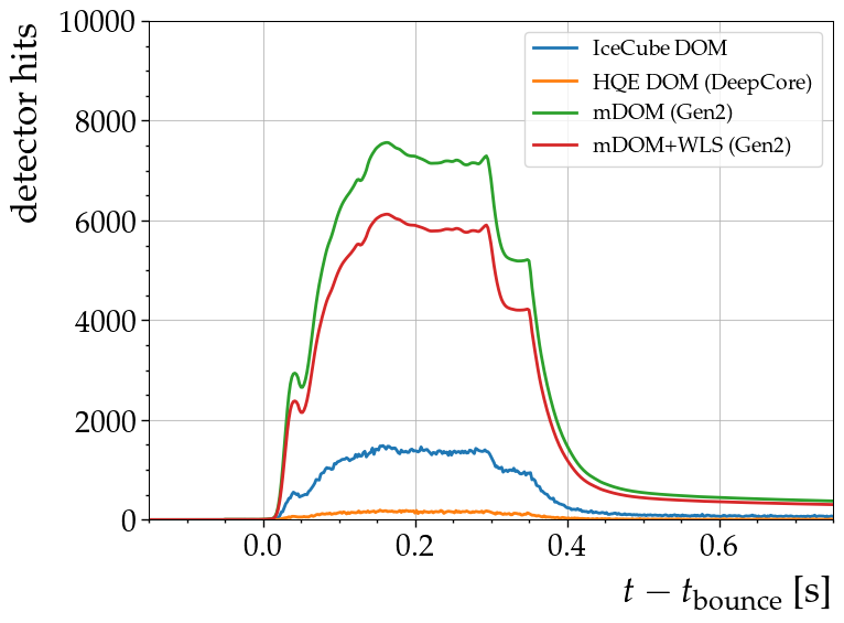
Add WLS Modules

In the Gen2 detector scope, using the add_wls=True argument will add wavelength-shifting modules to the Gen2 detector response.

The hits can be accessed as the ws subdetector.

sim_ws = Simulation(model=model,
                    distance=10 * u.kpc,
                    Emin=0*u.MeV, Emax=100*u.MeV, dE=1*u.MeV,
                    tmin=-1*u.s, tmax=1*u.s, dt=1*u.ms,
                    detector_scope='Gen2',
                    add_wls=True)
sim_ws.run()

t, hits_i3 = sim_ws.detector_hits(subdetector='i3', dt=dt)
t, hits_dc = sim_ws.detector_hits(subdetector='dc', dt=dt)
t, hits_md = sim_ws.detector_signal(subdetector='md', dt=dt)
t, hits_ws = sim_ws.detector_signal(subdetector='ws', dt=dt)

fig, ax = plt.subplots(1,1, figsize=(8,6), tight_layout=True)
ax.plot(t, hits_i3, label='IceCube DOM')
ax.plot(t, hits_dc, label='HQE DOM (DeepCore)')
ax.plot(t, hits_md, label='mDOM (Gen2)')
ax.plot(t, hits_ws, label='mDOM+WLS (Gen2)')

ax.legend(fontsize=14)
ax.set(xlabel=r'$t-t_\mathrm{bounce}$ [s]',
       ylabel=f'detector hits',
       xlim=(-0.15, 0.75),
       ylim=(0,10000));

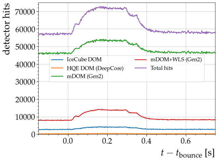
Plot the Sum of Signal + Background

bkg_i3 = sim.detector.i3_bg(dt, size=hits_i3.size)
bkg_dc = sim.detector.dc_bg(dt, size=hits_dc.size)
bkg_md = sim.detector.md_bg(dt, size=hits_md.size)
bkg_ws = sim.detector.ws_bg(dt, size=hits_ws.size)

bkg = bkg_i3 + bkg_dc + bkg_md + bkg_ws
hits = hits_i3 + hits_dc + hits_md + hits_ws

fig, ax = plt.subplots(1,1, figsize=(8,6), tight_layout=True)
ax.plot(t, hits_i3 + bkg_i3, label='IceCube DOM')
ax.plot(t, hits_dc + bkg_dc, label='HQE DOM (DeepCore)')
ax.plot(t, hits_md + bkg_md, label='mDOM (Gen2)')
ax.plot(t, hits_ws + bkg_ws, label='mDOM+WLS (Gen2)')
ax.plot(t, hits + bkg, label='Total hits')

ax.legend(loc='center', ncol=2, fontsize=14)
ax.set(xlabel=r'$t-t_\mathrm{bounce}$ [s]',
       ylabel=f'detector hits',
       xlim=(-0.15, 0.75),
       ylim=(0,75000)
);